Moser's tiling problem

Suppose you have an infinite sequence of squares of width \(n^{-1}\) for \(n=1,2,...\) The total area of all these squares will be \( \sum_n n^{-2} = \pi^2/6 \). Is it possible these squares can perfectly tile a rectangle of size \(1 \times \pi^2/6\)?

This question was posed by Meir and Moser in 1968. I learned about it from Terence Tao's blog post. If I had come to this problem cold, I would've estimated 99% the answer to be "no". You're essentially taking a random collection of puzzle pieces and hoping they somehow fit together. Sure, there are a lot of small squares that can be fit into the small gaps, but it'll never fit perfectly and each placement is going to create more weird shaped holes that need to be filled.

But somehow... it apparently is possible. In fact, the greedy algorithm will do it. Or so it seems. Paulhus (1998) was able to pack the first \(10^9\) squares, stopping there presumably because of computational limitations rather than because of running out of space. Remarkably, it seems that not only is tiling possible, but there is a surprising amount of flexibility. For instance, instead of squares you could consider rectangles of size \(n^{-1} \times (n+1)^{-1}\). And there are at least two different greedy algorithms that can be used:

Paulhus used the first algorithm. I prefer the second because it seems much more computationally efficient. The first requires maintaining a list of vacant rectangles that can grow quite large, and this list needs to be sorted so we can find the one that'll be just big enough to fit the next square. The second algorithm, on the other hand, essentially only requires a bit vector to record which squares have not yet been placed. We do still need to maintain a list of vacant rectangles, but this list never really grows beyond perhaps \(\log(n)\) because we are filling the smallest vacancies first and can discard them when they get whittled down to smaller than the smallest square we intend to place. (Clearly we are not placing infinitely many squares on the computer, so some cutoff needs to be chosen in advance.) Here's how it looks for placing the first 1000 squares: (source code)

The tail is easy

I've been trying to prove Moser's tiling conjecture, off and on, for a while now. Problem is, I get busy with other things for a few months and forget everything I learned about it. So I'm dumping my notes onto this page. Maybe it'll also inspire you to be interested in this problem.

It may be useful to start with the question: which part of the tiling is hard? Seemingly the hard part is fitting the larger boxes, and once those are taken care of there is a surprisingly large amount of free space to work with.

Specifically, if you look at the animation in the previous section, you will see that infinitely many times we cross a point where the remaining empty space consists of a single rectangle (this is particularly noticable near the end of the animation). At these points, we can ask how the size of this unfilled space compares to the size of the largest unplaced tile. Recall that the \(n^\textrm{th}\) square has width \(n^{-1}\). It's convenient to use the indices \(n\) as the unit of measurement for sizes. Each black dot in the plot below represents a point in the execution of algorithm #2 where the unfilled space consists of a single rectangle. The largest unplaced tile has width \(x^{-1}\) and the rectangular unfilled space is big enough to fit a square tile of width \(y^{-1}\). The takeaway message here is that after the initial tiles are placed, we have \(y^{-1} \gg x^{-1}\). That is to say, the unfilled space is vast and there is not even the most remote danger that we will be unable to place the next square. As long as the black dots remain below the green \(y=x\) line, we will not run out of space. It gets a bit tight in the beginning, but clearly by the time we get to \(x=100\) this hazard is easily avoided. The red dashed line is my guess at the asymptotic trend. It seems to fit remarkably well. (source code)

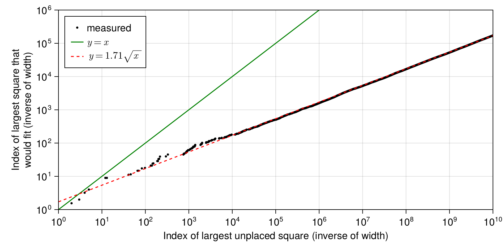
So why does this trend towards \( y = 1.71 \sqrt{x} \)? The constant factor is a bit of mystery, but I can explain the \(\sqrt{x}\) factor. Take a close look at the tail end of the animation at the top of this page. Starting from a vacant rectangle of width \(w = y^{-1}\) we place into the corner of this rectangle the largest unplaced tile, which has width \(x^{-1}\). We then place the next tiles above this one, filling up a whole column. Since \(x^{-1}\) is slowly changing when \(x\) is large, we can consider all these tiles to be about the same size. Therefore the number of tiles that can fit in this column is \(w x\). And the width of the large vacant rectangle decreases by the width of this column of tiles, which is \(x^{-1}\). But in the plot we are considering only the smaller of the width or height of the vacant rectangle. And to budge that, we need to fill not only the left column of the vacancy, but also the bottom row. This will take twice as many tiles, \(2 w x\). But not all tiles will be available. Many will have already been used by the algorithm for filling various small gaps. Let \(\rho\) denote the density of unused tiles. By using the next \(2 w x\) unused tiles, we are advancing the index of the largest unused tile by \( \Delta x = 2 \rho^{-1} w x \). And the size of the vacant rectangle decreases by the width of the row/column of added tiles, \( \Delta w = -x^{-1} \). This gives the differential equation \( \Delta w / \Delta x = -x^{-1} / (2 \rho^{-1} w x) = -\rho / (2 w x^2) \). Plugging into WolframAlpha gives the solution \( w = \sqrt{\rho} / \sqrt{x} \). Finally, we have \( y = w^{-1} = \sqrt{x} / \sqrt{\rho} \).

So this explains the square root in the fit \( y = 1.71 \sqrt{x} \) of the plot. And from this fit we can guess that the density of the largest unused tiles should be on average \( \rho = 1.71^{-2} = 0.34 \). Indeed this seems close to the truth: numerical experiments show it hovering around the range \( 0.36 \dots 0.42 \). We've related \(\rho\) to the slope of the fit in the plot, but why it should take this specific value is still a mystery.

Here is a histogram of the density of unplaced tiles of various sizes, as the algorithm progresses. Note that \(\rho\) is the density of the largest unplaced tiles (the tiles of lowest index), rather than the overall density. It's curious that this seems to tend towards a uniform distribution.

Though the density of unused tiles appears to approach uniformity, it most certainly is not random. Among the tiles from \(10^9 \dots 10^{10}\) (i.e., the last frame from the above plot), the used/unused status of a tile agrees with that of its predecessor 99.9637% of the time. This makes since because the filling algorithm tends to consume consecutive runs of tiles, stacking them into a column. Even filling in small gaps tends to involve laying down a sequence of tiles of as nearly uniform width as possible (i.e., consecutive runs).

How much room do we have to maneuver?

The previous section makes the point that it's the larger tiles that are hard to place, and once those are taken care of, there seems to be quite a bit of room for the smaller tiles (only in some intuitive sense, because in reality there is ultimately only exactly enough room to place them once all is done). This is good news, because it means we can have the computer place the largest 1000 tiles and then we craft some sort of proof that the remaining ones will fit.

Given how much space there is between the black dots and the green cutoff line in the plot from the previous section, it may seem we are already in a pretty good situation to attempt some sort of proof. But there is a major obstacle: the plot from the previous section takes snapshots at points in time where there is a solitary large rectangular vacancy. But in order to get to these points, the algorithm (we are running Algorithm #2) must have already placed infinitely many tiny tiles to fill up the other parts of the domain. Or, not quite infinitely many since for computational purposes we need to set some cutoff value. And this cutoff precludes any sort of proof because we really would need to consider the infinity of tiles in order to be sure that it all works.

Instead, we need to have the computer place only the first few largest tiles and then we come up with some sort of controllable way to place the rest of them. Something that facilitates some sort of proof (e.g., the collection of remaining tiles has property \(P\), which means we have room to place the largest one, and after that the remaing tiles still have property \(P\)).

As a first experiment, I had the computer place the first 5 tiles. There are then 5 rectangular vacancies. I was hoping to find some heuristic that would partition the remaining tiles to these 5 vacancies in such a way that the greedy algorithm could place them. The idea is to identify what sort of properties are needed of a tile collection in order to make it tileable to the rectangular vacancy. Clearly the area of the tiles must match the area of the vacancy, and each partition should have enough small tiles available to fill up gaps. But something more is needed. I couldn't get it to work.

This invites the question: is Algorithm #2 delicate? Does it work for some magic reason and any sort of perturbation breaks it? No. It seems quite resiliant. As an experiment, I had it first place the 5 largest tiles, then tile the remaining 5 vacancies in a random order. It always works. Or, instead of 5 you can do 100. It always works. This animation shows how these semi-randomized tilings look. Notice that there is always one of the five partitions that has a high density of very small tiles in the upper right corner (visible as a sort of white blob). That's the last partition to get filled, and this shows there is a surplus of very small tiles remaining at the end. This is encouraging, since the small tiles are valuable: they are what we use to fill up the small gaps. It seems we have more than enough of these available. (source code)

References

• Meir and Moser (1968) - where the problem was first posed.
• Paulhus (1998) was able to pack the first \(10^9\) squares.
• Terence Tao's blog post. Terence et al. proved you could tile if the squares shrink slower than \(n^{-1}\) and you discard the largest ones.
• Clive Tooth has nice animations showing the packing of the first millions of squares.
• Math StackExchange question by Clive Tooth - he explains the technique he used to pack the first \(10^{12}\) squares.
• MathOverflow question by Kaveh - answers give an overview of the literature.

<-- Home